Introduction
With the continuing increases in energy costs and the requirements of Biological Nutrient Removal (BNR), the design of the aeration system has become one of the most important aspects of the design of the activated sludge process.
With proper influent and operational data, process engineers can use a commercially available process simulator with activated sludge and aeration models to calculate temporal and spatial oxygen requirements. The calculated oxygen requirements can then be used to design the diffuser layout and calculate airflow requirements. The sizing of the air distribution piping, air control valves and blower are then based on the calculated airflows and a selected single point design pressure.
The single point design pressure is based on a single condition, but in reality, the actual pressure is dynamic, based on airflow and valve positioning. The large number of valve positions and influent conditions normally limits the engineer to only design for a single pressure, but the use of a single design pressure can lead to improperly sized equipment, which will promote operational difficulties and energy inefficiency.
Incorporating pressure losses and valve positioning calculations into the activated sludge model simulation allows the engineer to see the pressure and valve position changes as the influent process conditions change diurnally and seasonally so equipment can be sized accordingly.
This paper will introduce the process of calculating and incorporating pressure losses, blower speed and valve positioning into the activated sludge model simulation, quantify the control response for conventional and innovative control strategies, and demonstrate the benefits of flow-based blower control schemes versus pressure-based blower control.
Model Configuration
The basis of the model was an actual biological nutrient removal (BNR) wastewater treatment plant (WWTP) with a hydraulic capacity of about 19,000 m3/d (5 million gallons a day). The results of the simulation runs are based on this plant but have broad validity.
The commercially available software GPS-X by Hydromantis ESS, Inc. was used to perform the process simulation and pressure loss calculations. The aeration system model calculations were programmed into the GPS-X User File using Advanced Continuous Simulation Language (ACSL) statements; further information about GPS-X User Files and ACSL can be found in GPS-X and ACSL Reference manuals.
The aeration tank was modeled as a plug flow reactor; this model allows the reactor to be divided into numerous continuously stirred tank reactors (CSTR) in series. This, in turn, allows a great deal of operational flexibility in the model so that various conditions can be simulated. The reactor for this model was divided into eight (8) CSTRs in series. The dynamic inputs for the simulation were from actual sampling of influent flow, diurnal peaking factor, cBOD, TKN, and TSS data. The influent fractions were considered to be constant. The analysis was run for 259 days at a 15 minute time interval.
Aeration Model System Description
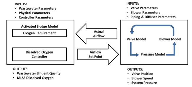
The aeration system model is a combination of valve, blower and pressure models that are all linked by the aeration system pressure (Psys). The models are solved iteratively until the actual airflow for each aeration zone is within the determined tolerance of the airflow set point, and the pressure model is balanced.
Figure 1: Activated sludge system and aeration system interaction
Valve Model
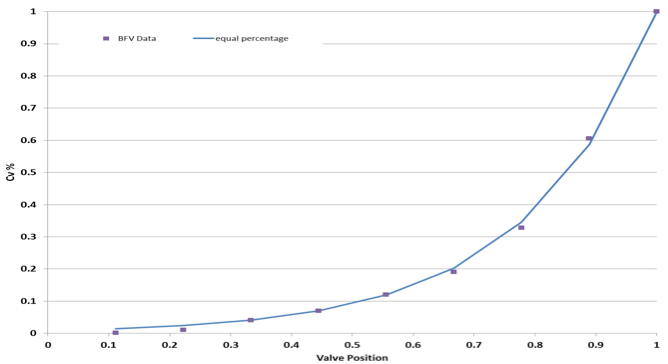
Within the aeration system the control valves are used to balance the airflow into the aeration zones. The most common control valves used for aeration control are butterfly valves. Control valves can be modeled by using flow coefficient (Cv) characterization curves. The Cv curve provides the relationship between the valve position and Cv. The curves are based on empirical data derived from laboratory testing done by the valve manufacturers. Figure 2 is an example of a Cv curve, and Equation 1 is used to describe the CV curve.
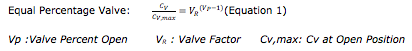
Figure 2: Butterfly Valve Cv Curve
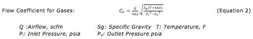
The definition of Cv is the amount of flow per unit pressure loss in units of gpm/psi. In regards to airflow, Equation 2 calculates Cv based upon the airflow and pressure on either side of the valve. Equation 2 can be rearranged to calculate the pressure loss across the valve (Pi –Po) at a specified airflow and valve position. The equation requires that the pressure loss across the valves is less than 10% of the inlet pressure (Pi) (Crane, 1991).
Blower Model
Blowers generate the airflow for the aeration system. Depending upon the type of blower, the airflow output is dependent upon the system pressure (Psys), blower speed, or inlet valve position and discharge vanes positions. For this paper only the positive displacement type blower was modeled, so only blower speed is needed to model the blower. Equation 3 was used to calculate the blower output based on percent of maximum speed (N). Depending on the control method of the blowers, the blower speed is modified until the control variable, airflow or system pressure, is within the control system dead band.

Pressure Model
To model the system pressure within the aeration system, pressure loss calculations are required for aeration piping, diffusers, and control valves. In regards to the control valves, the Cv Equation 1 is used to calculate pressure loss across the valve. The diffuser pressure losses are highly dependent upon the diffuser flux (scfm/ft2). Diffuser manufacturers can provide pressure loss versus flux curves. Data fitting analysis is used to generate a simple model equation. Calculating the pressure loss for the aeration piping can be fairly complex, because of multiple individual minor and pipe length losses required for the standard Darcy-Weisbach formula, but can be simplified by calculating pressure loss for one flow condition, then calculating a pressure loss coefficient that can be used for other flow conditions (WEF 2010).
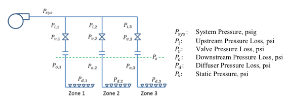
The sum of the minor pressure losses plus the static pressure becomes the system pressure (Psys) as shown in Equation 4. The sum of the minor pressure losses for each aeration zone must all be equal for the system to be considered balanced. Figure 3 is a depiction of all the minor pressure losses within a three zone aeration system.
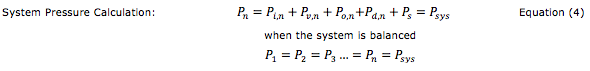
Figure 3: Aeration system minor pressure losses
Aeration Control Concepts
The goal of aeration control is to provide the required airflow to meet the current oxygen demand in each aeration zone while keeping the system pressure as low as possible. For this to happen, the blower control and the distribution control need to work together efficiently.
There are two methods for the distribution control to communicate to the blower control that a change in total airflow is required:
- The blowers are controlled to maintain a pressure set point requirement, which can be
- constant, independent of plant operating conditions, or
- dynamically calculated based on valve positions.
2. Airflow control, where the actual total airflow requirement is sent as a set point to the blower control.
1.a. Constant Pressure Blower Control At regular intervals, the aeration control system positions the air control valves to distribute the air to each aeration zone based upon the calculated airflow set point (typically using proportional-integral feedback control based on a dissolved oxygen error signal) for each zone. At the same time the blower control adjusts the output of the blowers to keep the system pressure within the specified dead band of the pressure set point. As the control valves open as airflow demand increases, the system pressure will drop and the blower control will then increase airflow to maintain the system pressure at the set point. The same control applies with the valves closing as airflow demand decreases, just in the opposite direction.
1.b. Dynamic Pressure Blower Control Dynamic pressure control is intended to promote lower system pressure by having the position of the most open valve (MOV) determine the system pressure set point. The MOV is controlled between two predetermined valve position set points (Jenkins, 2013). If the MOV is opened higher than the high set point, the system pressure set point is increased, increasing the airflow and forcing the valve to close to within the prescribed limits. If the MOV is closed below the low set point, the system pressure set point is decreased.
2. Flow Based Blower Control At regular intervals, the aeration control system sends a total airflow set-point to the blower control, and then positions the air control valves to distribute the air to each aeration zone based upon the calculated airflow set point for each zone.
The valve control includes dynamic most open valve logic to promote low system pressure by having one of the control valves become the most open valve (MOV) at 90% open and allows the other control valves to seek their position to meet the airflow requirements. When a control valve that is not the MOV is calculated to be at greater percent open than the MOV, then that valve becomes MOV, and the previous MOV will be able to close.

Results
The model demonstrates a correct and verifiable response to steady state input conditions, and a stable, repeatable response to variable loading conditions, so it is suitable for evaluating and comparing aeration system designs and aeration control schemes.
Changes in blower, valve and pipe sizing were all tested to determine their effects on system performance and operating efficiency. Only the results for testing the aeration control concepts are shown in this paper.
Control system comparisons
A simulation was run for each of the three aeration control logic concepts described above; all simulations used the same airflow piping, valve sizes and airflow rates. The control responses were tuned in the model to provide best possible performance. The simulations were run for seven days with a 15 minute control step interval.
1.a. Constant Pressure Control The constant pressure simulation had a system pressure set point of 7.6 psig, with a 0.05 psig dead band on the blower control.
1.b. Dynamic Pressure Control The dynamic pressure simulation had the MOV set points at 60% and 45% open with a system pressure set point change of 0.05 psi with a 0.05 psi dead band on the blower control. Simulations were run at various MOV position set points to try to optimize system pressure for the dynamic pressure control. At first the MOV set points were increased to drop the system pressure but control became unstable, with the MOV bouncing between the set points due to the sensitivity of the valves to pressure changes at high open ranges. Then the MOV set points were spread apart, but that resulted in performance similar to a constant system pressure set point.
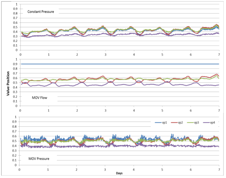
2. Flow Based Control The flow based simulation had the MOV set at 90% and the blower control had a 30 scfm or about 1 % of the blower capacity dead band. Figure 7 shows the valve positions and system pressure of the simulations.
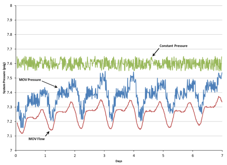
The flow based control valve positions were the most open, showing aeration zone 1 as the MOV at 90%, while the other three control valves were between 40 to 70% open. Next, the dynamic pressure control showed valve positions between 30 and 60% open. Last, the constant pressure valve positions were between 30 and 50%. The system pressure is dependent upon the valve positions, which is seen in the system pressure comparison figure. The constant pressure control is the highest at 7.6, moving within the dead band of the set point, while the flow based control is lowest between 7.1 and 7.4 psig without the operational noise of the system pressure dead band. Using the extended time period simulation data, the system pressure and airflow results were used to calculate blower power requirements. Compared to constant pressure control, dynamic pressure saved 3% in aeration power, while flow based control saved 5% and provided more stable valve responses.
Figure 4: Valve positions and system pressure for different aeration control methods
Conclusions
The design of the aeration system has become one of the most important aspects of the design of the activated sludge process, but process engineers only have commercially available process simulators with activated sludge and aeration models to calculate dynamic process requirements, not the actual equipment requirements for an aeration system.
It was demonstrated that the process of calculating and incorporating pressure losses, blower speed and valve positioning into the activated sludge model allows the engineer to see them change as the influent process conditions change diurnally and seasonally, so equipment can be sized accordingly.
Using the combined models for control valve sizing, estimating the pressure requirement for the blower, and comparing the dynamics of three different types of aeration control methods was also demonstrated.
At this point, the aeration system model could not be compared to actual operational data. A comparison would be valuable, and should be done to determine the overall accuracy of the model. However, the valve, blower and pressure models were developed using methods already used in design, which gives confidence that the models as used in the paper would provide an accurate design tool.
For more information contact Tilo Stahl, BioChem Technology, tel: 610-768-9360
References
Crane Flow of Fluids. USA: n.p., (1991). Print. Technical Paper No. 410.
Jenkins, Tom. "Aeration Control." E-mail interview. 25 June 2013.
WEF. Energy Conservation in Water and Wastewater Treatment Facilities. Alexandria, VA: WEF, Water Environment Federation, 2010. Print.
To read more articles on Wastewater Treatment, visit www.airbestpractices.com/industries/wastewater