Introduction
Facility managers, how would you like the peace of mind from knowing the system you had installed or modified is thoroughly tested - to the same degree as a new production line? How would you like to be confident that the money you spent is still paying back benefits, year after year?
Air compressor dealer personnel, how would you like to know that your installed compressed air systems are “bullet proof”? That the coordination of parts and pieces function as a whole, and do not “drift” out of optimal condition by random gremlins nibbling away at them?
Auditors and utility DSM energy engineers, how would you like to know that the systems you post-verified or retro-commission are going to stay in that condition? You know that in many of your projects, one little change in adjustment, and efficiencies will evaporate.
All three project stakeholders need to have one agreed-upon robust methodology for commissioning a system, and the teamwork to do it correctly the first time. That is the intent of this series of articles.
Background
In Part 1 of this series on commissioning, I made the case that compressed air systems are typically not commissioned properly at the time a retrofit project is implemented. Further, I made the point that proper commissioning would make most controls “re-commissioning” projects unnecessary. This does assume that some measurement metrics are visible that point out the slippage, if even a well-commissioned project falls into disrepair.
In Part 1, I suggested the following definition:
“Compressed air system commissioning is the process for measuring, testing, adjusting, and documenting that the performance of an entire compressed air system achieves the target system efficiencies (scfm/kW as a whole and for each piece of equipment) in all load regimes and potential failure modes.”
This article will attempt to start to describe a general methodology for commissioning that should cover most compressed air systems projects. In a series of articles, I will discuss four aspects of commissioning: measurement and data-plots, testing and adjusting, and documentation. This article will be focused on measurement and data plots.
Measurement
Measurement is seen as costly and time-consuming. If over-designed, that is a justified concern. It is also typically seen as a separate service provided by a separate entity. There are skill specialization issues that often make that necessary. I will propose a measurement methodology that assumes permanent, low-cost instruments are installed, accented by temporary measurement. Economics will put boundaries on the money spent for measurement. See my June 2015 article in this journal, “Determining the Economic Value of Compressed Air Measurement Systems.”
The minimum measurement devices needed for proper commissioning are as follows:
1. Permanently installed:
- Input AC electrical current, one leg, on each and every compressor and dryer package (except no-energy dryers like HOC or heatless regenerative). These are current transmitters (CTs) and cost about \$300/each. This is current before a VFD, not after.
- Compressor discharge pressure(s), ideally one point. These cost about \$300/ea.
- System discharge pressure(s), ideally one point
- Data-logging system. There are a variety of systems on the market, from simple data-loggers for under \$1,000 to fully-integrated SCADA systems. See below for a discussion.
Permanent measurement recommendations in this article might or might not be sufficient to meet a utility-required post-verification. Temporary monitoring might be needed to accent it.
2. Temporarily installed (if justified economically, permanently installed):
- Flow, after dryer(s). I recommend simple, low cost thermal mass type like flow meters, about \$3000/each.
- Indication of dryer purge flow, purge pressure.
- Power meter(s), spot-measured or permanent (depending on utility requirements). There are many options, and are usually loaned or rented from an utility, auditor, or equipment vendor. These cost about \$1000/each.
If there is sufficient budget, the temporary devices should be permanently installed.
Data-logging Discussion
Why have permanent logging at all? Most projects don’t. The main reason is to provide a basis for real-time indication and maintenance of performance, called “continuous commissioning” by some. At a minimum, it lowers the cost for having an outside auditor provide performance analysis for the customer. The technology sold in the project and available at the customer’s site affect what type of data-logging is practical. I will present an ideal method and a couple alternatives, for when you can’t achieve that ideal. Once you make that technology decision, you are “in bed” with it for the life of the system, short of a new retrofit project! Your monitoring technology choices are going to be limited by your prior control system choices. And those were economically-governed as well. Sometimes they were not done ideally, but you need to work with what is there.
Get the monitoring installed as a part of the project, not after everyone is gone and paid. If the plant network part is not done yet, often the laggard in a project, local PLC downloads of data can suffice for the commissioning phase. As a part of that installation, validate the zero-energy states of your sensors, and either automatically offset them in your system, or in your Excel analysis file. This is particularly important for pressures.
Data-logging System Alternatives:
1. Sequencer (or master control system) with continuous data-logging included. This would include memory, local visualization, and a way to output data for analysis, ideally continuously and automatically. This can be done multiple ways, depending on the type of sequencer:
- Stand-alone air compressor OEM sequencer with data-logging embedded, proprietary hardware. There are several on the market, some with trend data. Prices vary considerably, but are generally from \$10k to \$40k.
- Custom 3rd-party management systems. There are two families, PLC-based and embedded-controller based. The PLCs don’t trend data in general, and require a separate piece of software on a PC and sometimes a server. Prices are dependent on many project-specific issues, but usually start at about \$25k and can go to over \$100k.
2. Separate “smart” data-loggers. These are configurable monitoring systems that have “widgets”, or calculation function blocks, that do some real-time analysis to simplify data, and export data to a separate PC. An auditor is probably needed to supply and program the logger. These systems cost about \$2k to \$5k.
3. Simple data-loggers. The simplest logging systems that can’t do any real-time calculations or connect to a network are cheaper. These systems cost about \$1k to \$2k. But one audit to upload and analyze the data is multiple times that cost.
Set the sample rate sufficiently fast to catch the system transients. There is no “rule” that is perfect. But it is impossible to troubleshoot a pressure cycling problem that happens in 20 seconds with a 30-second sample rate! I like to have about 3 sample rates or more per pneumatic event I am trying to measure. During the first part of commissioning, the system will not be dialed-in, and some of those events are quick. As a result, you will probably like a 10-second sample rate or better at first.
Data Trends and Plots
These plots are currently not available on any commercially-available compressed air monitoring systems, so they will need to be made in Excel separately. One example of a data scatter plot that I do for every compressor is as follows:
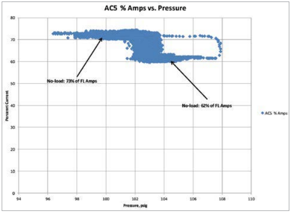
1. Air Compressor Amps vs. Pressure. This shows how the air compressor responds to pressure, basically an air compressor controls plot. See Figure 1 for an example of load-unload control. This came from a project where the air compressor was a centrifugal, and was in full blow-off instead of fully unloaded. No-load power was quite high, over 400 kW, and couldn’t be modified at the time. The compressors were centrifugals and would essentially blow-off instead of unload.
Figure 1. Load-unload Compressor Controls Plot
Smart Data-logging Functions for Calculating Key Performance Indicators
These can be programmed into some smart logging systems or programmed in Excel, requiring a skilled compressed air auditor. The essential values are as follows:
- Power. If real kW is not monitored, just current, calculate power from current using two power-factor values, full and no-load. Power = Amps x Voltage x 1.732 / 1000 x PF. Add up all power.
- Air Compressor Flow. An estimate can work if flow meters are not in the permanent system. Assign flow based on compressor flow based on performance literature and motor current. A threshold is used (if current is over loaded, and under max) and then a two-point calculation (flow proportional to current, full and min flow). Calculate total compressor flow by summing individual compressors’ flow.
- System Efficiency. Individual and aggregate compressor and dryer flow/power ratios.
- Unloaded Waste. Program a reasonably accurate estimate of total no-load power. Create a variable called “no load power” for each compressor. For starters, assume a 60% power factor for no-load condition. Use a threshold to indicate that unloaded condition is occurring, Amps < 50% of full load, for instance. Then, for those periods, calculate no-load power. At no-load, kW is about 0.50 x the current for 480V. So 40 Amps no-load would be about 20 kW. Add up all compressor and dryer no-load power to a “total no-load power” variable.
- Blow-off/vent/purge Waste. Program a reasonably accurate estimate of wasted flow, in scfm. This can be done with a pressure transducer on a vent valve pressure signal (for centrifugal compressor) or on the purge pressure for a dryer. Linear assumptions between two points can be used, with thresholds for zero and max flow. Add up all that waste as one value, total wasted air. In our view, it is not cost-effective to install a permanent flow meter to measure something that you want to be zero.
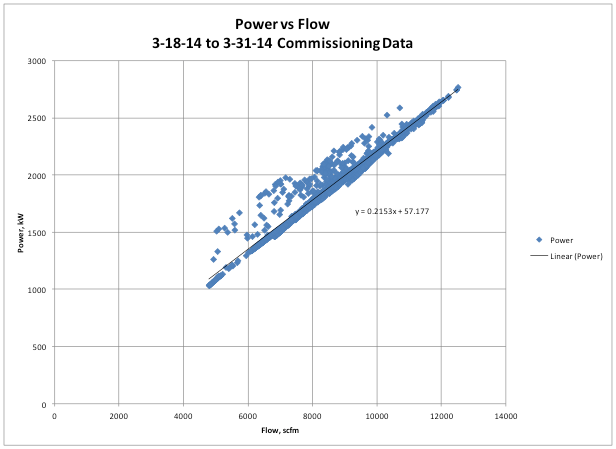
- Total Power vs Total Flow. See Figure 2 for an example. The total power and flow values need to be averaged over about 5-10 no-load cycles, maybe a 10-min or longer smoothing interval. Then, they are correlated and plotted on an X-Y plot. The slope and intercept can be calculated in Excel. The intercept is the total power of the system at no flow, a very important key performance indicator. Ideally this is zero.
If you wanted one performance indicator to determine if an air compressor controls project was operating efficiently, it would either be total no-load power or total blow-off. The project that Figure 2 comes from had a total of 4,000 hp of compressors on line. The no-load power could have overwhelmed the system efficiency, so master controls had to minimize it. Even though there were four 700 hp compressors, two of which had a “no load” power of > 400kW each, we got the average total system no-load waste to 21 kW.
Figure 2 comes from the same project that had the potentially high no-load power described in Figure 1. System controls tuning reduced the amount of time that the compressors were in the no-load condition, giving the total system a very efficient performance curve, almost zero power at zero flow. That “Y intercept” is a very important measurement of system efficiency, influenced by largely by the total no-load power.
Figure 2. Total Power vs. Flow Scatter Plot
Other Useful Data Trends
- Number of no-load air compressors running at any one time. This tells you situations where the system is not tuned well. Usually caused by over-shoot and undershoot of pressure. A zoom-in on data can identify timer adjustments that can remedy the problem. See Figure 3 for an example of a target sequencer system that would start too many compressors, then have to stop unload and stop them, creating a large pressure swing. The no-load power peaks as the pressure drops, then goes to zero as all compressors are loaded and pressure shoots back up. The overall no-load power is an indicator of system performance, but this is a diagnostic trend to determine why it was too high (before tuned).
- Pressure differential and dryer flow. Can be used to widen the sequencer pressure differential and avoid system pressure dips at max flow. See Figure 4. This system had the VFD sensing point ahead of the dryer and the sequencer downstream, no ideal. But we were able to avoid nuisance starts of fixed speed compressors by widening the sequencer pressure differential or moving the sensing location to downstream of the dryer.
Figure 3. Data Trend Showing Pressure Over-undershoot
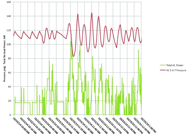
Figure 4. Data Trend Showing Dryer Pressure Differential as VFD Loads Up

Conclusions
Measurement of compressed air shouldn’t just be a separate “auditor” function that is before and after a project. Measurement needs to be integrated into commissioning of the system as a whole. In addition it should be part of the long-term measurement to show that it stays in tune. For robust commissioning to happen, a reasonably low-cost measurement system needs to be put in place during the project, some key performance indicators calculated from it, and some data plots made to identify what root causes are contributing to less than ideal performance. Then, the system can be adjusted and optimal performance achieved and sustained.
To read Part 1 of this article please click here. To read Part 3 of this article, please click here.
For more information, contact Tim Dugan, tel: (503) 520-0700, email: Tim.Dugan@comp-eng.com, or visit www.comp-eng.com.
To read more Compressed Air System Assessment articles, please visit www.airbestpractices.com/system-assessments.